Alice is tasked with improving the performance of an algorithm. She remembers hearing that a new accelerator has been released, which can perform operations 30% faster than the one her team is using. She pushes her boss to invest in this new accelerator, succeeds, and excitedly plugs it in, but performance remains the same… and her boss is not happy.

At the same time, Bob is tasked with doing the same for a different algorithm. He carefully dissects it and after a month of work he produces an algorithm that improves the cache hit rate by 80%! Excitedly, he deploys the new algorithm, but the performance is also the same… Bob feels like all that effort went to waste.

Despite their effort, why don’t Alice and Bob see returns in performance?

Optimizing the right thing

Optimizing a program is full of hairy real-world constraints and limits. Fundamentally, we are limited by the work our algorithm needs to do (how many operations we need to perform) and the how fast we can do it (how many operations can we perform per second). As we dive into these these, we uncover all sorts of headaches relating to software implementation details of the various frameworks we use as well as hardware details of how our components behave.

In determining which headache to face next, it is useful to have a high level map of where our fundamental bottleneck lies. Here, we try to study performance bottlenecks at a fundamental level, so we can try to avoid Alice and Bob’s mistakes. Lets consider the following:

Scenario

We have a task to perform, detailed by an algorithm. It requires performing a fixed number of operations on some data. We carry out the operations with an accelerator, to which we feed the data.

What determines our performance?

1. Obviously, how fast we perform the operations, but also
2. how fast we read and write data

FLOPs FLOPS and FLOP/s - Alice’s story

A floating point operation (FLOP) is the most basic building block of our algorithms. A very natural way to measure how much work we are doing is to count how many of these we are carrying out. Of course, we have to perform the operations on something, so we need to feed the accelerator with data. The rate at which we perform operations is somewhat independent of the rate at which we are able to read/write the incoming/outgoing data.

If we can move data infinitely fast, then it is clear that a faster accelerator improves our performance, being able to perform operations at a higher rate. Alice’s thinking is that, at the end of the day, we have a certain number of FLOPs that need to be performed, as dictated by our algorithm. As long as this is fixed, the only way to improve performance is to carry them out faster.

However, if our data rate is not high enough, we are effectively starving our accelerator of data. No matter how fast it is, it cannot perform operations on nothing, and neither can a faster accelerator.

FLOP and derived metrics

Somewhat unfortunately, the existing abbreviations and their inconsistent usage make an initial reading into this extremely confusing. To avoid that, I’ll try to be very clear with what I mean with each term:

FLOP - A floating point operation.

FLOPs - The plural of FLOP. Sometimes mistaken for a measure of performance, this is rather a measure of the amount of work carried out. (Think distance)

FLOPs/s or FLOPS - FLOPs per second. This indeed is a measure of performance. (Think speed)

Thus, the runtime of our task when we don’t pay for data movement will be $\text{runtime} = \frac{\text{FLOPs}}{\text{FLOPs/s}}$

Thinking in units

When thinking about this type of work, we often try to derive different metrics building on the ones we have. As a hint to doing this, I often found it useful to think in units as a guidance for the quantities we need.

In the simple example above, to get runtime we want our final unit to be seconds. If we have FLOP/s, we need to flip the seconds to the top and remove the FLOP, thus we need to divide by something with a unit of FLOP

Arithmetic intensity - Bob’s story

Let’s then consider the data rate. Let’s forget about how fast our accelerator performs operations for now, and assume it is infinitely fast. Do we now take 0 seconds to finish? As Alice has learned, unfortunately not… We can’t perform operations if we don’t have any data to perform them on, no matter how fast we are.

In the same way we described the total work to be done from the perspective of operations to be carried out, using FLOPs, we can describe it with the amount of data that needs to travel in and out of the accelerator, in Bytes. Here, not all algorithms are equal - some are more “data hungry” than others.

Combining these two constraints gives us a fundamental insight into our algorithm, known as arithmetic intensity:

Arithmetic Intensity

$AI = \frac{\text{FLOPs}}{\text{Bytes}}$ This measures how many operations we perform for each byte we move. We divide FLOPs by Bytes, rather than the other way around, as the rate at which we perform operations is orders of magnitude larger than the rate at which we read and write data, so we are quite interested in doing as much (useful) work as possible for each byte we need to move.

We can recover some quantities we are interested in based on this formula. If we know the bandwidth (BW: how many bytes we move per second), we can recover the effective FLOP/s we will obtain with our infinitely fast accelerator: $\text{Effective FLOPs/s} = \frac{\text{FLOPs}}{s} = \frac{\text{FLOPs}}{\text{Bytes}} \times \frac{\text{Bytes}}{s} = \text{AI} \times \text{BW}$

And thus also the expected runtime of our algorithm: $\text{runtime} = \frac{\text{FLOPs}}{\text{Effective FLOPs/s}} = \frac{\text{FLOPs}}{\text{AI} \times \text{BW}}$

Thinking in units (cont.)

The above calculations are slightly more contrived, but we can think in units to keep it simple. I try to frame it like this: given units of FLOP and Byte, if you want to get FLOP/s out, you need to introduce the time unit, and remove the Byte unit.

Putting it together

We must combine the facts that our accelerator is not infinitely fast at performing operations, and that we must pay the cost of moving data. Depending on the AI, we are either bound by one constraint or the other: “Compute bound” or “memory bound”. Why is AI the determining factor for this?

Let’s look again at the equation for effective FLOPs/s above. Assuming a fixed BW, as we increase AI, we directly increase FLOPs/s. This is true, until we reach the peak FLOPs/s of our accelerator. From this point, no matter how much we increase AI, our FLOPs/s are capped by the compute capacity of the accelerator.

We can now introduce our roofline model, which plots the metric we really care about, effective FLOPs/s, against the factor that determines our constraint, AI.

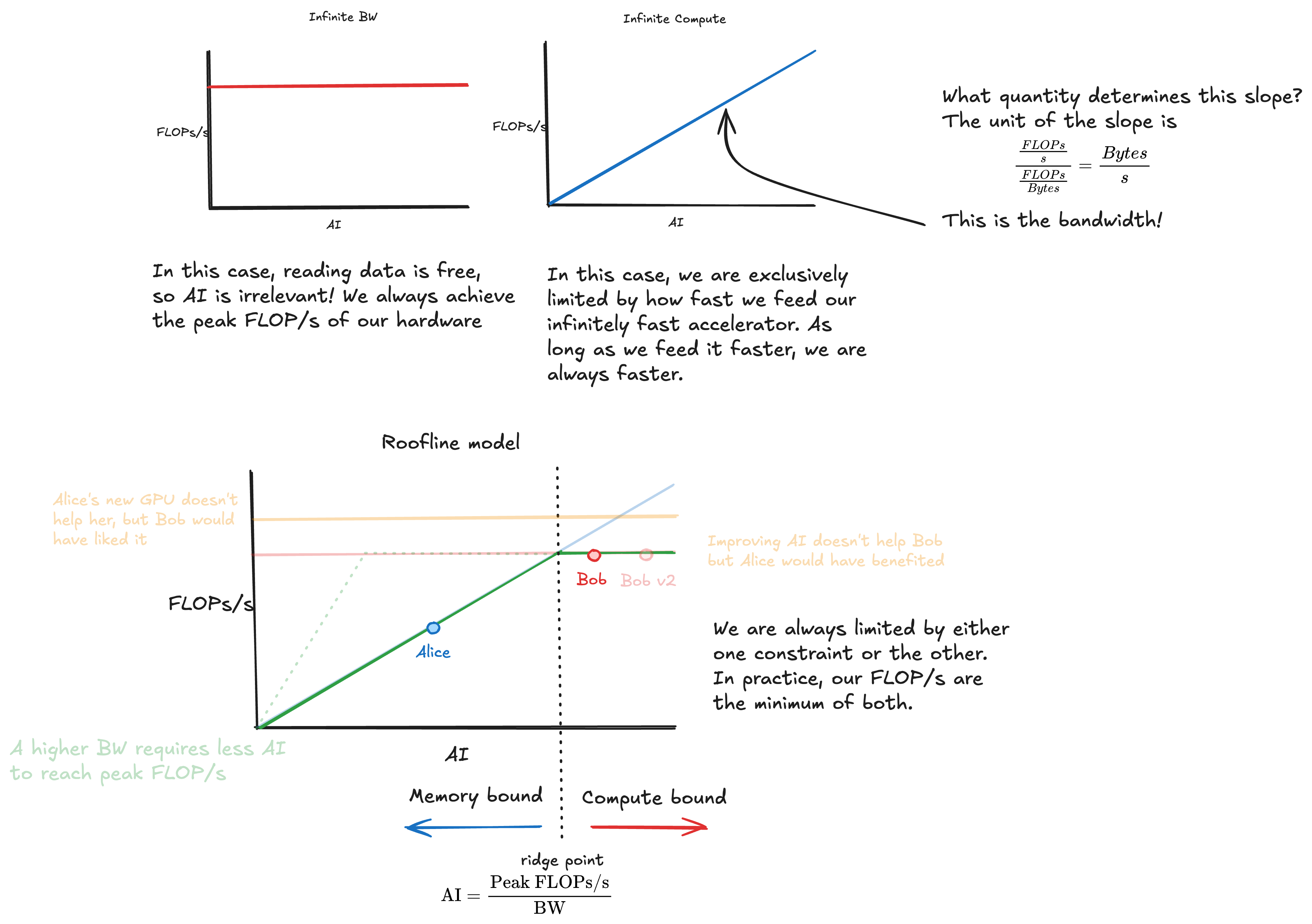
The ridge point is where the diagonal memory line meets the compute ceiling. It occurs at AI = Peak FLOPs/s / BW. Operations with AI below this are memory-bound; above it, they’re compute-bound.

AI on the x-axis

In the begining I found it confusing to reason about this chart due to AI being on the x-axis. This is how I came to terms with it:

• The y-axis is the Effective FLOPs/s, the metric we care about.
• Effective FLOPs/s can never be higher than the peak FLOPs/s of the accelerator, so we have this horizontal line capping us.
• We want to reach this performance, by enabling the accelerator to perform the operations at this rate. The two things we need to know are how much data do i need to perform an operation, and how fast can i provide this data. AI describes the first part, and BW determines the second.
• The interplay of how fast we can feed the data (BW), how much data the algorithm needs per flop (AI) and the maximum FLOP/s, determines our performance $\min (\text{FLOPs/s}, \text{AI} \times \text{BW})$

Back to Alice and Bob

We now understand why our characters’ efforts were misguided.

Alice

• Alice’s algorithm was memory bound. Buying a new accelerator increased the peak FLOPs/s, but for Alice that was never the bottleneck. (If the accelerator has higher BW however, this could help - see the dotted green line)
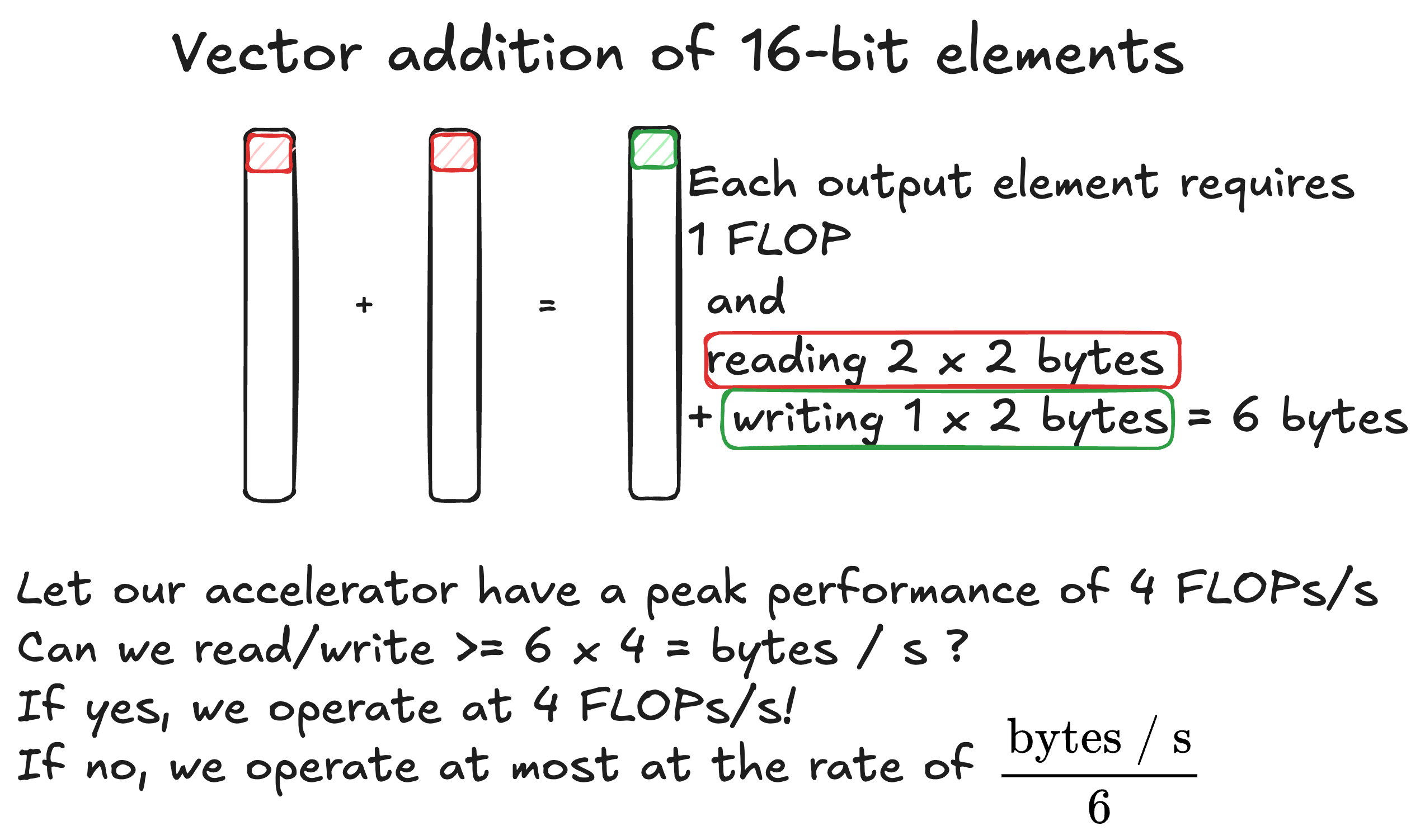
• An example of this algorithm might be the addition of very large vectors. Each compute operation on an element requires 2 reads and 1 write.

Bob

• Bob’s algorithm was compute bound. While Bob’s algorithm now accesses memory faster, it remains bound by the peak FLOPs/s the accelerator can deliver.
• Bob’s algorithm may contain large matrix multiplications, for example. For a matrix multiplication of size N×N, we perform N³ multiply-add operations but only need to read 2N² elements (two input matrices) and write N² elements (output). As the matrix grows, the number of operations scales faster than memory accesses: O(N³) operations vs O(3N²) memory accesses. This is why large matrix multiplications tend to be compute-bound. $O(\text{reads \& writes}) < O(\text{operations}) \Leftrightarrow O(3 \times N^2) < O(N^3)$

Practical implications

What does all this mean for practitioners? The first takeaway should be that its critical that we understand what the bottleneck is before we start optimizing. This is a generally good idea across engineering disciplines. When optimizing program performance specifically, that means knowing where you sit on the roofline charts. Many tools, such as NCU, have an option to plot this for you.

If you are memory-bound, increase your AI! Kernel fusions, larger batch sizes and activation recomputation are common paths forward.

If you are compute-bound, that means you’re already getting the best use out of the compute you’re paying for! You can splurge for that fancy new accelerator without feeling bad.